ChessCoach
– Chris ButnerA neural network-based chess engine capable of natural language commentary
High-level explanation
Classical and neural network-based chess engines
Classical chess engines such as Stockfish have improved steadily over decades and led the field in playing strength for most of that time. However, their fundamental structure and core methods have remained largely unchanged. Neural network-based chess engines represent a radical departure in evaluation and search methods. They have only become viable at the highest level of play quite recently, and much is still unfamiliar about their workings. It may help to dive into the differences between classical and neural network-based engines, and explore how these networks are used to play chess.
The AlphaZero-style neural network is the heart of the ChessCoach project. All search and training functionality is built around it. The neural network has two functions: firstly, to evaluate a position, estimating the probably that the side to play is winning (called value), and secondly, to estimate the probability that each legal move in a position is the best (called policy). In a game like tic-tac-toe, looking at an unfinished game and making an evaluation is not necessary because the engine can see to the end of all lines of play. In chess or Go, even after 7 or 8 back-and-forth piece moves (called halfmoves or plies), there are too many unfinished games to keep track of, and the tree of possibilities keeps growing exponentially for 70 or so more plies. The search needs to find a good place to cut things short and make what is called a static evaluation.
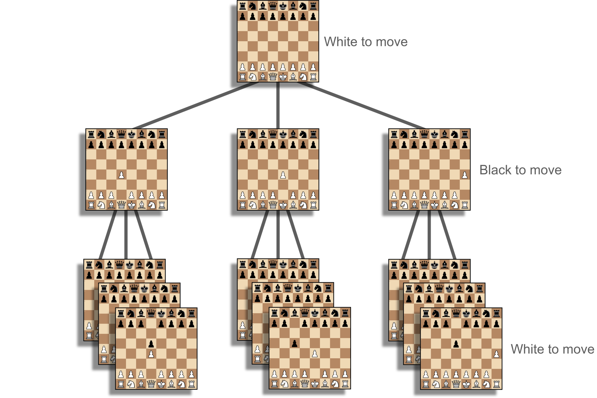
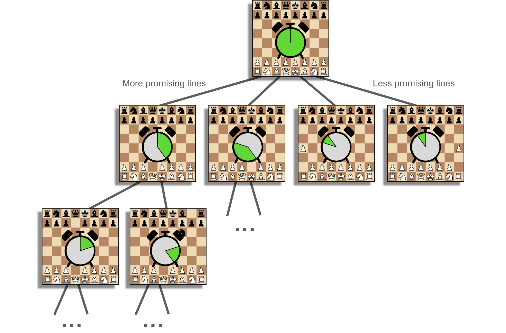
Classical engines assume that both players will always alternate making the best move, so they expand the tree as far as they can then make static evaluations at the leaves, before deciding which line of play is the best that each player can do (see Figure 1). This is called the principal variation. Generally, the deeper an engine can search this tree without missing anything important, the stronger it will be. Most of the progress in classical engines during the previous few decades has come from pruning this tree; that is, working out which moves and possibilities do not need to be calculated because they are not good enough, too good, not interesting enough, and so on, and skipping them. This starts with iterative deepening, move ordering and alpha-beta pruning and extends to hundreds more techniques. These are the giants' shoulders to rebuild or build upon when working on a hobby engine.
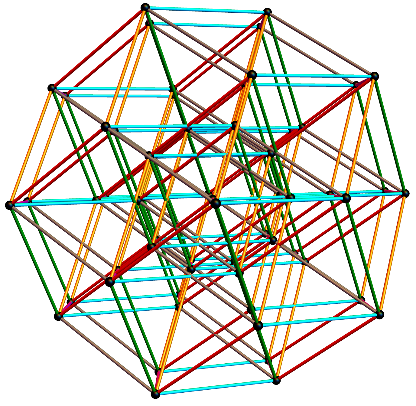
Neural network-based engines such as AlphaZero, Lc0 and ChessCoach take a different approach, firstly by making much more complex (but slow) static evaluations, and secondly, by making these evaluations at every position in the tree, rather than just at the leaves. One basic reason for this being necessary is because the second function of the neural network – the policy calculation – is needed to explore outward from each position. However, AlphaZero has an appealing explanation for why it also helps with overall evaluations. A neural network's static evaluation is a highly complex non-linear function as opposed to a classical engine's linear function. It is a messy curve as opposed to a straight line, but in a highly dimensional space. Think of a point, then a curve, then a curved surface, and then keep following that process for 250 more steps (see Figure 2). Non-linear functions can be much more accurate but also much more inaccurate. Rather than representing an entire line of play with just one final evaluation, neural engines blend all evaluations along the way. This is akin to a human player saying, "this position looks great for me but also very dangerous".
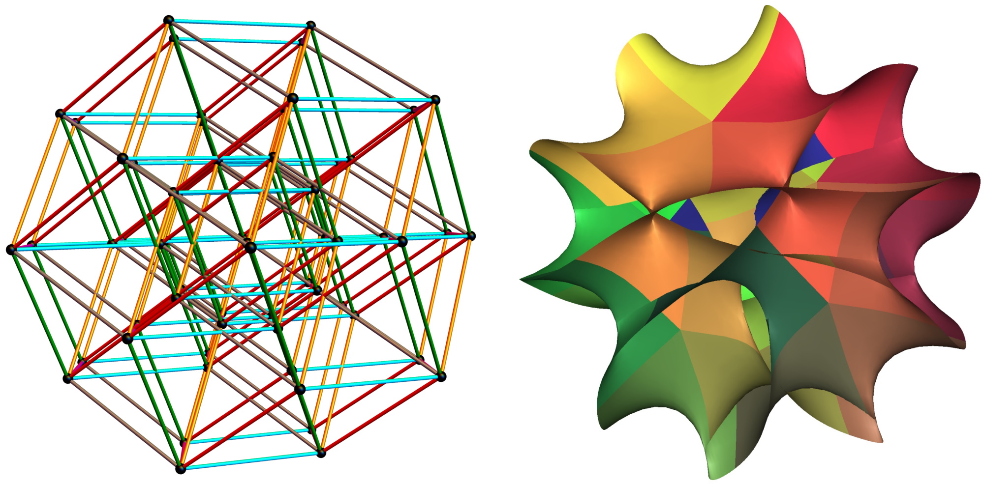
Figure 2: Linear vs. non-linear 6-dimensional spaces projected to 3 dimensions
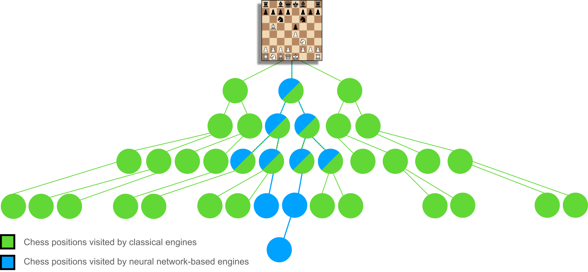
Using this blending approach requires a different kind of search algorithm. Classical engines generally use alpha-beta pruning, an optimized variation of what is broadly a minimax approach, assuming best play from each side and placing absolute trust in every static evaluation. AlphaGo Zero and AlphaZero's innovation here was to instead use Monte Carlo tree search (MCTS) driven by the policy output of the neural network. The policy takes the place of classical pruning and achieves deeper, more accurate searches by guiding MCTS towards the most promising lines. Despite evaluating the slow neural network at every position, these types of engines can still beat classical engines by taking a more "human" approach, finding regions of the search tree that classical engines underestimate and ignore, in a "Tortoise and the Hare"-type situation (see Figure 3).
Neural network
Neural networks are really just big, parallel number-crunching machines, which is why they are perfectly suited to GPUs and Tensor Processing Units (TPUs) (although our own brains are immensely more efficient). This sounds like something that computers and classical engines do normally, so you might ask, what is special about neural networks? The answer is that the architecture of the network and the types of calculations are designed to be very calculus-friendly, and often take biological structural cues to create a deterministic, stable and fast way to train the entire network at once. Like a teacher in a classroom, we can give the network a problem to work on, compare its answer to the real one, and use calculus to update every small part of the network to give a slightly better answer next time. The small parts are called weights and are just decimal numbers.
Of course, there is no guarantee that taking a lot of small steps will eventually allow a network to give correct answers. Explorers taking this approach could become mired in numerous gullies taking what looks to be the easiest route, without seeing the bigger picture. Training of neural networks is highly sensitive to architecture, data and methods, and this is even more pronounced for chess because it is difficult to label "correct" answers. Who is to say what is the perfect evaluation of a position or policy for move selection?
Luckily, the team at DeepMind worked through a lot of these details with AlphaZero, presumably at great expense, and emerged with an architecture and set of methods based on convolutional neural networks as well as recent innovations such as residual connections and batch normalization. Convolutional networks take small, trainable filters and slide them across images, just like applying a blur in Photoshop. However, the output is interpreted as gathered data rather than as a visual medium. This is an efficient way to recognize interesting features and applies well to 2D grid-based board games like Go and chess.
In an approach inspired by our own visual cortex, stacking these filters in sequence creates a hierarchy of complexity, with earlier layers recognizing lines, corners and gradients; middle layers recognizing squares, spheres and patterns; and later layers recognizing sedans, burgers and Labradors. This sliding, hierarchical approach is efficient and powerful because it allows us and neural networks to instantly recognize upside-down faces, cars to our left and right, and small and large string instruments as the same type of thing without duplicating all of that machinery many times.
It is easy to see how this can apply to pattern-recognition over the chess board. However, you might think that convolution filters are too clunky over a small, discrete 8-by-8 grid as compared to a large, continuous image, or that a layered sliding approach may be too slow to understand long-range effects from queen, rook and bishop moves. Nope – works great.
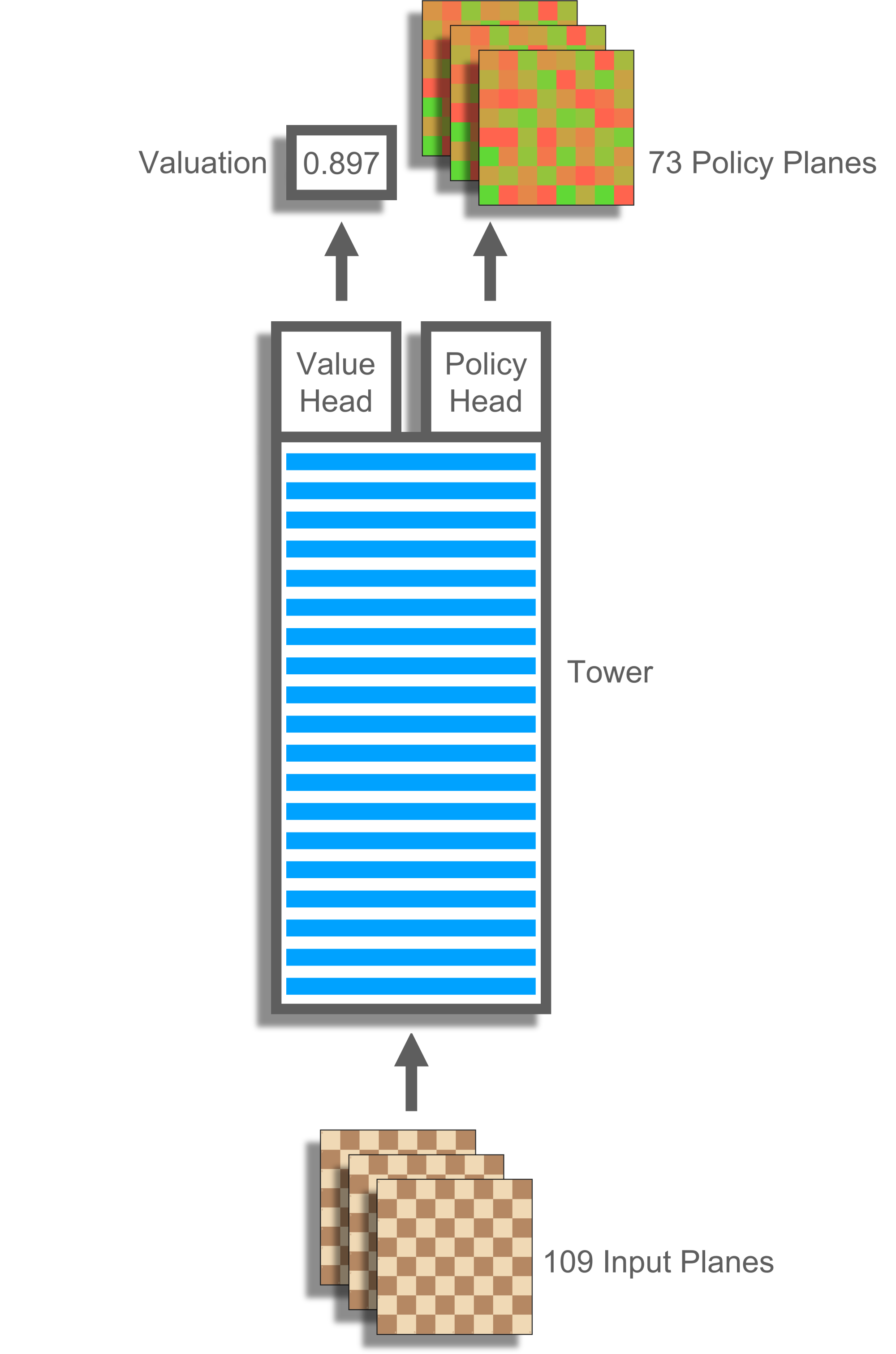
ChessCoach's primary neural network is almost identical to that of AlphaZero's. It takes as input a number of planes. These are 8-by-8 grids representing features such as "current player's pawns", "other player's knights", "three positions ago was a repetition" and "seven moves until a 50-move draw". The inputs pass through a deep tower of convolutions before reaching two separate heads (see Figure 4). One head calculates value, a single number. The other calculates policy, a set of 8-by-8 planes representing probabilities for different moves. Attaching these two heads to the one body saves calculation time and helps regularize the network. Using limited computational space for multiple tasks means that the network is less likely to over-specialize and "see phantoms" in positions that it is less familiar with.
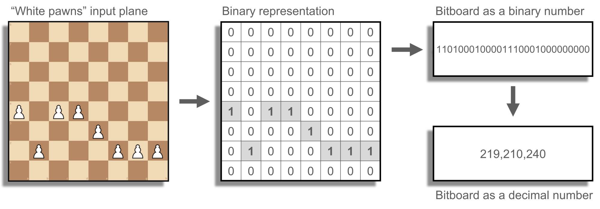
Each cell in the 8-by-8 input planes is a one or zero because chess is a very discrete game, so these planes can be packed in transit into 64-bit whole numbers. This saves space and time and aligns perfectly with the way high-performance code manages chess boards, positions and rules; that is, using bitboards (see Figure 5).
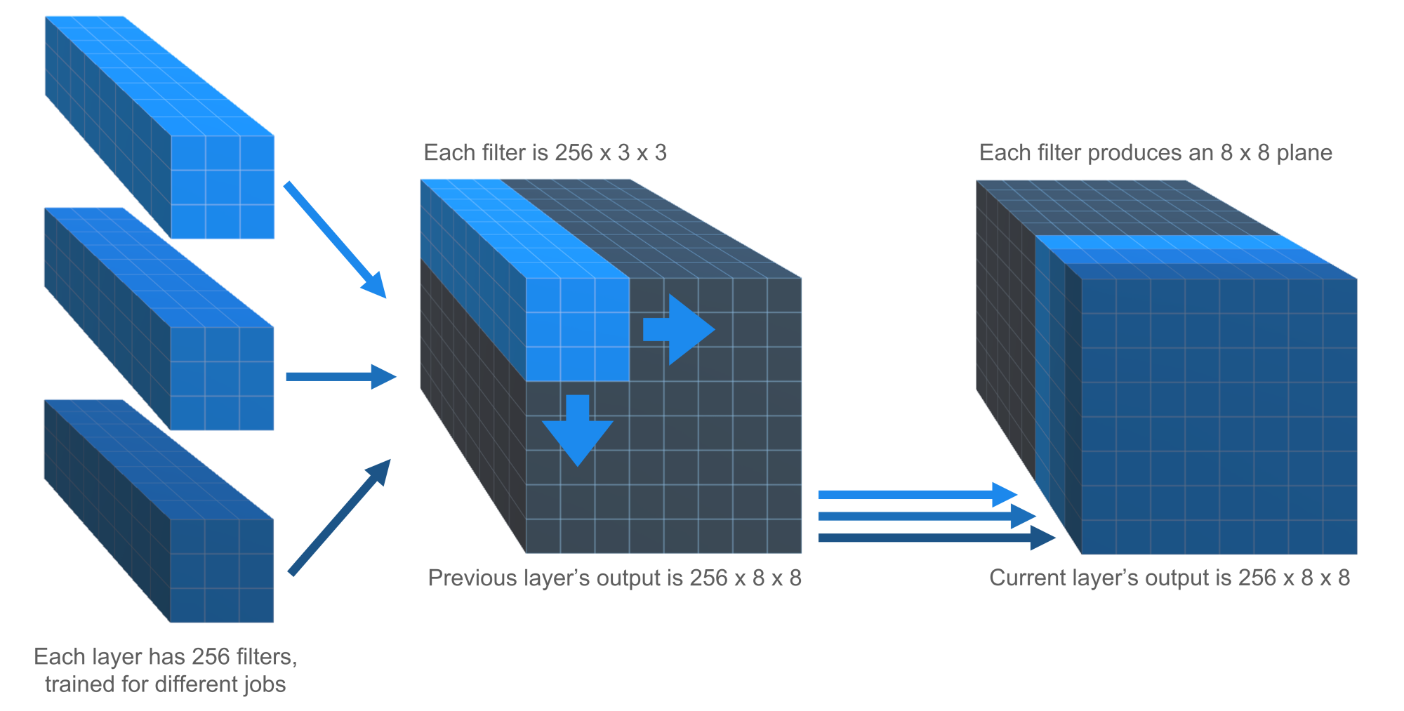
ChessCoach starts with 109 input planes; that is, a collection of 109 × 8 × 8 ones and zeros. The last 8 positions supply 13 planes each for pieces and repetitions, and 5 additional planes are included for castling rights and the 50-move rule. At each layer in the network, convolutions slide 3 × 3 filters over the 8 × 8 chess board. However, a large amount of data needs to be gathered; for example, in the early stage, features such as "my pawns are lined up"; in the middle stage, features such as "my knight can capture their queen"; and later, features such as "my position is solid". Because of this, each layer has its own set of 256 convolution filters trained for different jobs, and each of these filters is not just 3 × 3 in two dimensions, but 256 × 3 × 3 in three dimensions, sliding over the output of each of the previous layer's different filters (see Figure 6). So, at each layer there is a set of 256 × 8 × 8 decimal numbers that represents the total learned so far about the position. Considering that each number can vary in one dimension, from very negative to very positive, the network can be considered to be thinking 16,384-dimensionally.
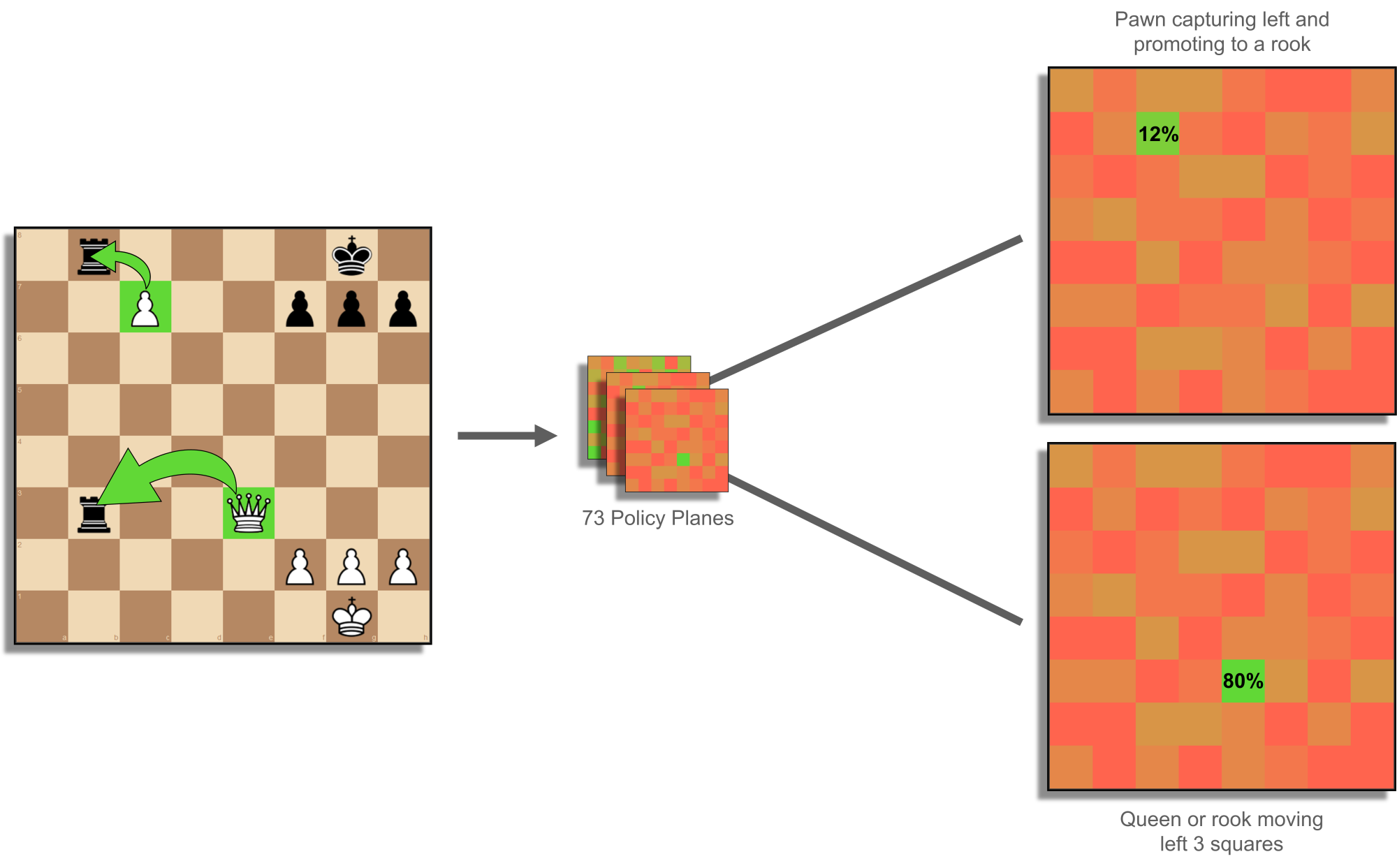
In the end, the value head returns a number such as 0.99, an almost-certain win, and the policy head returns a set of 73 planes comprising 73 × 8 × 8 decimal numbers. Each cell on the 8-by-8 grid represents the starting point of a move, and the plane represents the type of move (see Figure 7); for example, a pawn capturing left and promoting to a rook, or a queen or rook moving left 3 squares. There are 56 types of "queen" moves (up to 7 squares away in 8 directions), 8 types of knight moves, and 9 types of underpromotions. Kings, queens, rooks, bishops and pawns all make "queen" moves. Unfortunately, the outputs as valuations and probabilities are decimals and cannot be packed into bitboards, instead feeding straight into the search algorithm.
Search
Monte Carlo methods in computing take problems that are normally too difficult to solve, and apply randomness to find approximate solutions through statistics. Traditional Monte Carlo tree search (MCTS) uses random playouts, simulating a number of games to completion using random moves. With enough playouts (or rollouts), the search can get a feel for how good a position is, based on potential outcomes. However, what people often do not realize (understandably) about AlphaGo, AlphaGo Zero and AlphaZero is that their MCTS implementations are deterministic until sampling and multi-threading are introduced. AlphaGo (Silver et al., 2016) uses a trained fast rollout policy (in combination with a value network) but introduces randomness by sampling from it. AlphaGo Zero (Silver et al., 2017) and AlphaZero (Silver et al., 2018) use sampling for move selection during self-play only, not tournament play, and most importantly do not use playouts at all, relying entirely on the value head of the neural network. These latter algorithms are defined by the "glue" between their neural network policy and node selection during tree search, called PUCT, and I believe it is better to name the algorithms this way.
PUCT – derived from PUCB (Rosin, 2011) and UCT (Kocsis & Szepesvári, 2006), each deriving from UCB (Auer, Cesa-Bianchi & Fischer, 2002) – stands for Predictor-Upper Confidence bound applied to Trees and is a calculation used at each node in the search tree to decide which move to examine. This choice is often framed as a multi-armed bandit problem, referencing a hypothetical problem wherein a gambler is trying to maximize profit from multiple slot machines with unknown payout rates. The problem comes down to an exploration vs. exploitation trade-off. The gambler wants to maximize their profit and exploit high-paying machines as often as possible but needs to invest in exploring and discovering those high-paying machines, especially when it takes multiple plays to accurately calculate payouts.
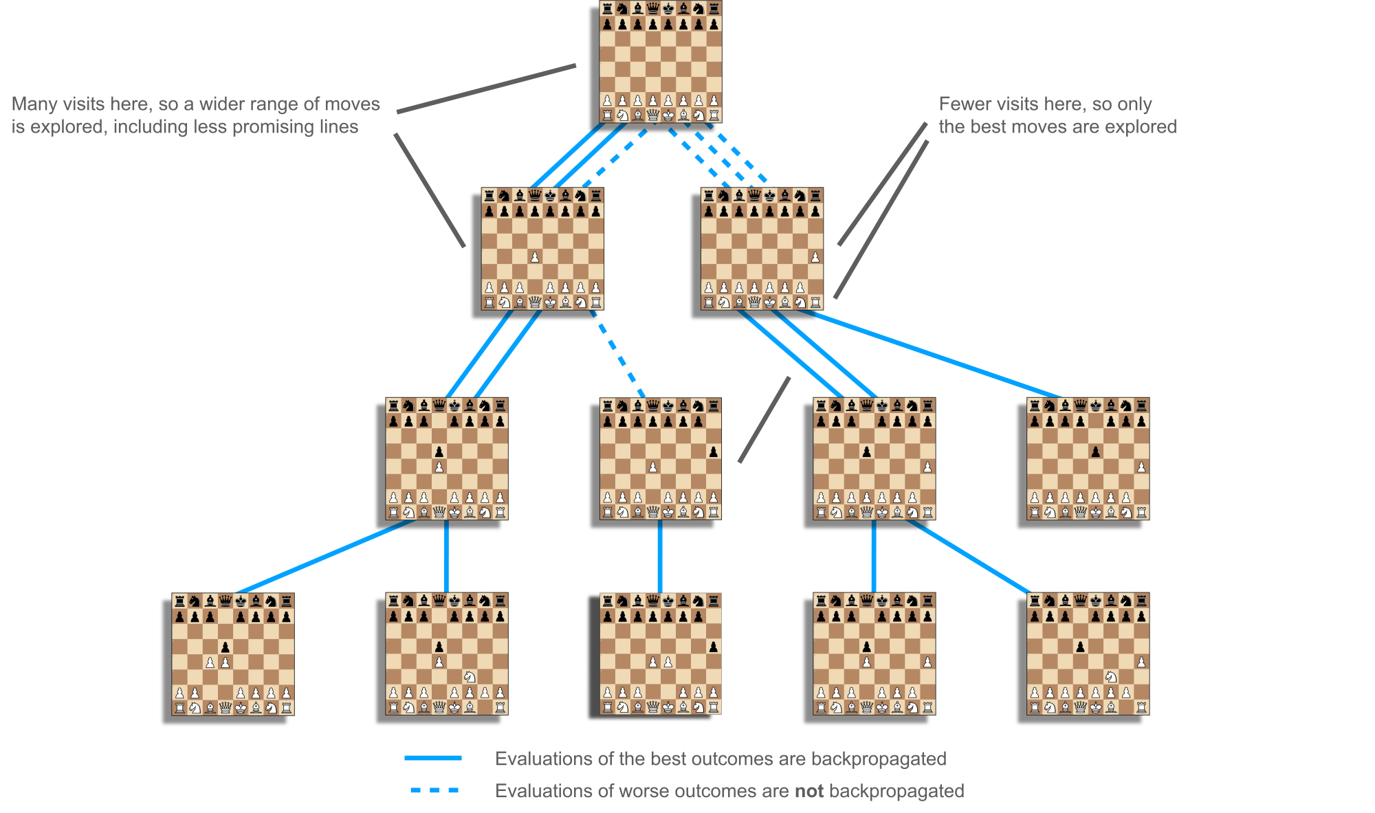
In chess, the same trade-off arises in an abstract sense. Search time is a limited resource that is invested into various positions to find winning game outcomes (see Figure 8). It is important to keep visiting offshoots of the most promising line in order to accurately calculate value, by generally aggregating more potential outcomes, seeing more clearly as the simulated game nears completion, and discovering tactical surprises. However, it is also important to explore a variety of moves to discover and exploit the best one. The key is to grow a search tree by running many simulations, each time making exploration vs. exploitation choices until reaching a new position, then statically evaluating it and averaging that value back into all ancestors. In this way, positions throughout the tree are valued according to the aggregate of potential outcomes they allow.
Auer, Cesa-Bianchi & Fischer (2002) and Kocsis & Szepesvári (2006) show that with enough simulations, mostly exploiting the best known move but occasionally showing optimism for less-explored moves, the results of the search converge to those of minimax, as used in classical engines. The upper confidence bound (UCB) metric is used to quantify exactly how optimistic to be and still converge. It would be dangerous to explore too much because the aggregated value would include evaluations from too many poor moves that didn't have to be made: a position with one winning move and five losing moves could look quite bad and be passed over. Rosin (2011) gives a method for assigning more exploration resources to more promising moves when this information is somehow known ahead of time, and this is exactly what the trained policy head of the neural network is for. However, AlphaZero uses a metric different to Rosin's for this bound, so I will call theirs AZ-PUCT and use this term interchangeably for both the metric calculation and overall search algorithm, rather than the confusing MCTS.
One discrepancy you may notice in treating tree search for chess as a hierarchical multi-armed bandit problem is that the gambler is concerned with overall profit: the sum of all winnings, even from low-paying machines, minus costs. This is optimizing for cumulative regret: minimizing the sum of each instance of regret corresponding to the difference between the best possible payout and actual payout for that play. PUCT, UCT and UCB concern themselves with cumulative regret, and this can work quite well. However, a better optimization target when thinking about tree search in chess is simple regret, wherein after a search period, a single instance of regret is incurred based on a single, final play.
Bubeck, Munos & Stoltz (2010) show that "[t]he smaller the cumulative regret, the larger the simple regret", which is a surprising result. However, they go on to demonstrate better outcomes when aiming to minimize cumulative rather than simple regret even in one-shot scenarios such as making a move in chess, unless the total number of simulations made is sufficiently high. Minimizing cumulative regret requires at most logarithmic exploration as a function of simulation count, and minimizing simple regret requires linear exploration, while maintaining exploitation. AZ-PUCT makes an interesting compromise here, choosing to grow exploration with the square root of simulation count, in combination with an additional factor that starts at 1.25 and grows logarithmically after a delay.
Tolpin & Shimony (2012) similarly suggest a square root exploration incentive, and additionally propose a two-tiered approach to minimizing regret by considering simulation counts higher and lower in the search tree; for example, minimizing simple regret at the root and cumulative regret lower. Lc0 discusses a concrete proposal mirroring this approach. However, Pepels, Cazenave, Winands & Lanctot (2014) contend that accurate search relies on each player making the best response to their opponent's moves, and therefore, moves deeper in the tree should use the same algorithm as at the root, requiring a consistent application of any tiered approach. Their proposed method, H-MCTS, is such, relying on sequential halving (Karnin, Koren & Somekh, 2013) in higher parts of the tree as they reach a sufficient simulation count, and UCT in lower parts of the tree, with the boundary extending non-uniformly as required. Sequential halving operates by repeatedly eliminating the worst half of the moves currently under consideration, but requires an upfront simulation budget; that is, always knowing the search time in advance and not stopping early. It also requires simulating in batches. These factors make implementation quite conditional and complex.
With ChessCoach I introduce a new method, SBLE-PUCT, based on Linear Exploration and Selective Backpropagation, applied via elimination. The primary danger of exploring too much is that value is diluted in ancestors. SBLE-PUCT tempers this by breaking the assumption that evaluations are always propagated all the way back to the root. In its metric form, it encourages minimization of simple regret after a delay by adding a linear exploration term to AZ-PUCT. However, in its algorithmic form it only allows backpropagation of value while AZ-PUCT alone would have made the same choice of move, up to a small delta, and breaks the chain when this stops being the case. This allows wider exploration without damaging the upper search tree, while still accurately calculating value in previously neglected sub-trees and allowing unexpectedly good moves to be propped up and exploited by AZ-PUCT (see Figure 9). Elimination is used as in H-MCTS to avoid wasting too much time but is applied one simulation at a time, without requiring batching. The elimination only applies to the linear exploration term, and the search performs effectively with no or partial elimination for infinite or stopped searches.
Self-play and training
Neural networks training themselves through self-play is a form of reinforcement learning. Multiple actions (moves) are taken in an environment (a chess game) with the goal of maximizing rewards (winning) and learning to do so better in future. Various forms of reinforcement learning have been applied to chess. Prior to the AlphaGo family, the most recent was Giraffe (Lai, 2015), which uses a form of reinforcement learning called TDLeaf(λ), used in the KnightCap engine (Baxter, Tridgell & Weaver, 1999) and based on TD(λ) (Sutton, 1988).
Algorithms like TDLeaf(λ) are used because attributing rewards to individual actions in a game like chess is a difficult proposition. The game result, win, loss or draw, is the only thing that really matters, but not every move directly causes it: often a single blunder decides a chess game. The result is also just one data point, so multiplying it out to each move creates thinly stretched information and strong correlation, which can be detrimental statistically. Additionally, it is computationally expensive to play a full game of chess in order to gather just one game result. Reinforcement methods instead often decay attribution by weighting training rewards more heavily for moves closer to the result. Another alternative is aiming to predict an intermediate result such as the engine's own evaluation of the position following the move.
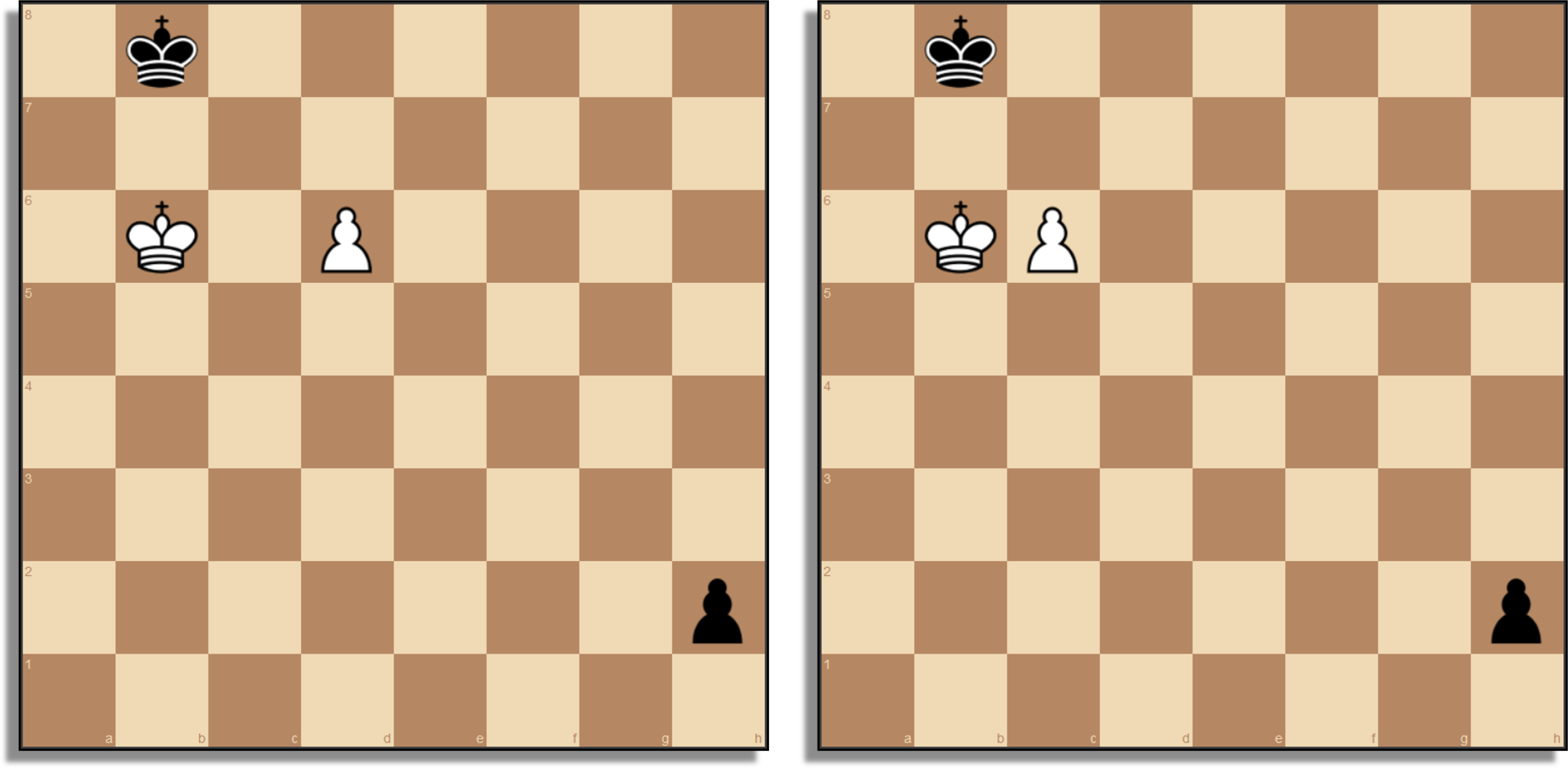
Chess is a particularly difficult target for reinforcement learning and machine learning in general because tactical surprises appear frequently (Ramanujan, Sabharwal & Selman, 2010). Making a tiny change to a position, such as moving a pawn one square over, may change a win to a loss (see Figure 10). Neural networks struggle to deal with non-smooth surfaces like this during training, especially when making predictions for positions they are unfamiliar with, and require vast quantities of data to compensate.
One of AlphaZero's greatest achievements was overcoming these challenges and developing a set of methods that elegantly ensure convergence despite wrapping a rather brute-force core. The game result is fully attributed to every move when training the value head, and the shape of the search tree, driven by the policy head, goes back into training the policy head. The value training is the dream of machine learning: taking the entirety of the raw data, throwing it into a black box without any human bias, and getting a good result out. The policy training is more complex as while it does involve more biased systems, parameters and tuning, policy predicts much more information and is more sensitive to the non-smooth, tactical nature of chess. As a result, its convergence up to 3000+ Elo strength is even more surprising.
After numerous failed attempts in ChessCoach to improve policy training through accelerated learning and tactical insight, I concluded that AlphaZero's policy feedback cycle works because of three reasons:
- It has high inertia, only allowing its shape to change slowly.
- It maintains some uncertainty through mean reversion, not growing over-confident and stubborn.
- It generally refrains from trying to understand tactics, instead leaving that to search.
I believe that a policy network/head that can maintain an understanding of position alongside tactics is possible but will require a much larger network, improved hardware, and perhaps a new type of architecture. That is not to say that current networks cannot spot forks or sacrifices. However, consistent reconciliation of general principles with reasoned exceptions is beyond current networks, and attempts too far along these lines instead lead to instability and worse positional understanding.
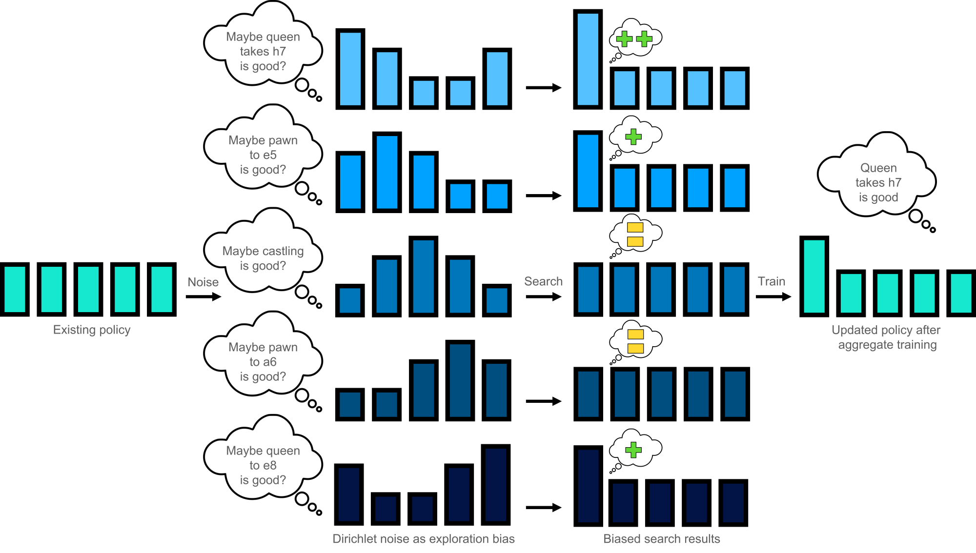
For every move in a self-play game, ChessCoach follows AlphaZero's process and uses the network's policy output as a prior probability distribution in a Bayesian sense, aiming to arrive at a posterior distribution with which to train future networks using SBLE-PUCT search (which effectively collapses to AZ-PUCT during fast self-play games). After 800 simulations, the number of visits from the root to each possible move form a new distribution as the training target. AZ-PUCT has a desirable property in that while the best move will eventually get most of the visits, at lower simulation counts the distribution just follows the original priors. Compared to the millions used during tournament play, a figure of 800 simulations is tiny. It allows for relatively faster data generation, but also provides a suitable trade-off between allowing good moves to prove themselves, with some help, and keeping the distribution from reshaping too fast, as in (a) above. Help for undiscovered moves is provided in the form of Dirichlet noise, a gamma distribution, which blends into the prior distribution at 25% weight. Across many games, this noise will eventually give each move an initial boost. However, since training effectively aggregates billions of positions, moves have to prove themselves worth the boost, since they are equivalently dragged down some of the time instead. This serves the desired uncertainty and mean reversion of (b) above. Because of the relatively small simulation budget, aggregation across positions, and tactical volatility between similar-looking positions, the network tends to absorb universal truths rather than exceptions, as in (c) above. Figure 11 summarizes these processes.
ChessCoach also follows the AlphaZero training schedule, generating 44 million self-play games and feeding 700,000 batches of 4,096 positions into training the neural network by providing targets for the value and policy heads derived from those games. AlphaZero completed its training in 9 hours using 5,000 Version-1 Tensor Processing Units (TPUs). With ChessCoach, I had free access to approximately 50 v3-8 TPUs by the end, generously provided through Google's TPU Research Cloud (TRC) program – an astonishing amount of computing power – but training still took multiple weeks for the final run, and months to reach that point. It is a little disappointing how many training games are needed and how much processing power is required, and I was not able to achieve much improvement. Projects such as Lc0, and Fishtest for Stockfish have had significant success sourcing computing resources from the wider community. I believe few-shot methods more akin to human learning will be necessary for breakthroughs in future, both in game-playing and general machine learning.
With ChessCoach I tried many different techniques, most existing in literature but not yet applied to chess, to improve the speed or quality of training, with most ending in failure. The main survivors were knowledge distillation (Hinton, Vinyals & Dean, 2015), stochastic weight averaging (SWA) (Izmailov, Podoprikhin, Garipov, Vetrov & Wilson, 2019), auxiliary training targets (Wu, 2020; and Prasad, Abrams & Young, 2018) and warmup. Some techniques for tournament play may also have helped training speed and quality.
Training was implemented to be flexible, scaling from single-GPU up to multi-GPU and v3-8 TPU scenarios. To achieve this, the base training batch size was set to 512 rather than 4,096 and multiplied along with learning rate by the number of devices; correspondingly, the total training steps were set to 5,600,000 rather than 700,000 and divided by the number of devices. On a v3-8 TPU, the schedule becomes AlphaZero's (although with 8 × 512 batches instead of 64 × 64, which does affect batch normalization, regularization and convergence). Code and configuration refer to ChessCoach steps; however, in this documentation I will use AlphaZero steps for easier comparison.
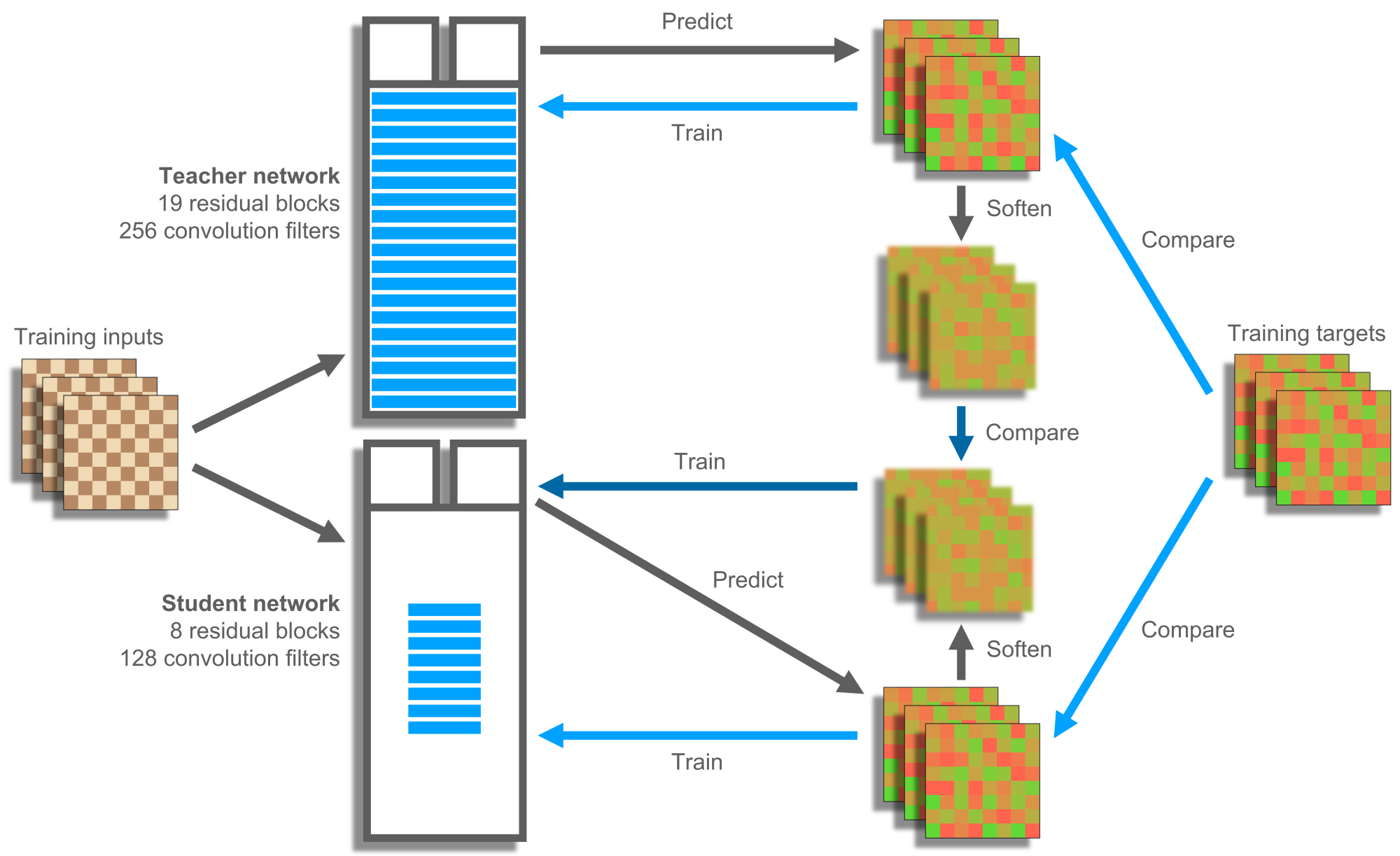
The most resource-intensive part of the training schedule is generating self-play games; hence, speeding this up is an excellent target. I used knowledge distillation to train a large, teacher network with 19 residual blocks (each consisting of two convolutional layers with a skip-connection) and 256 convolution filters in parallel with a small, student network with 8 residual blocks and 128 convolution filters. The teacher learns directly from the training data, but the student learns from a combination of the training data and the teacher's knowledge (see Figure 12). This sounds counter-productive because the teacher is still learning from the training data itself; however, benefits derive from softening the teacher's knowledge by applying temperature when distilling it to the student, dampening overconfidence for best moves and amplifying policy predictions for worse moves. From this the student can discern the texture of the distribution; for example, rather than just being told that queen-takes-h7-with-check is good here and everything else is bad, learning that most checking moves are good here. Ordinary training for a network is a little like being told to learn everything a Grandmaster knows simultaneously, whereas additional texture can help get across individual "concepts" in a human sense to build into the hierarchical network structure. I am not confident that knowledge distillation helps in ChessCoach in a statistically significant way, but in any case, I see no downside in the data using the student network to generate self-play games up to at least 100,000 training steps. Other projects have used this technique in a loose sense by continually training two networks and leap-frogging the larger, once it starts out-performing the smaller.
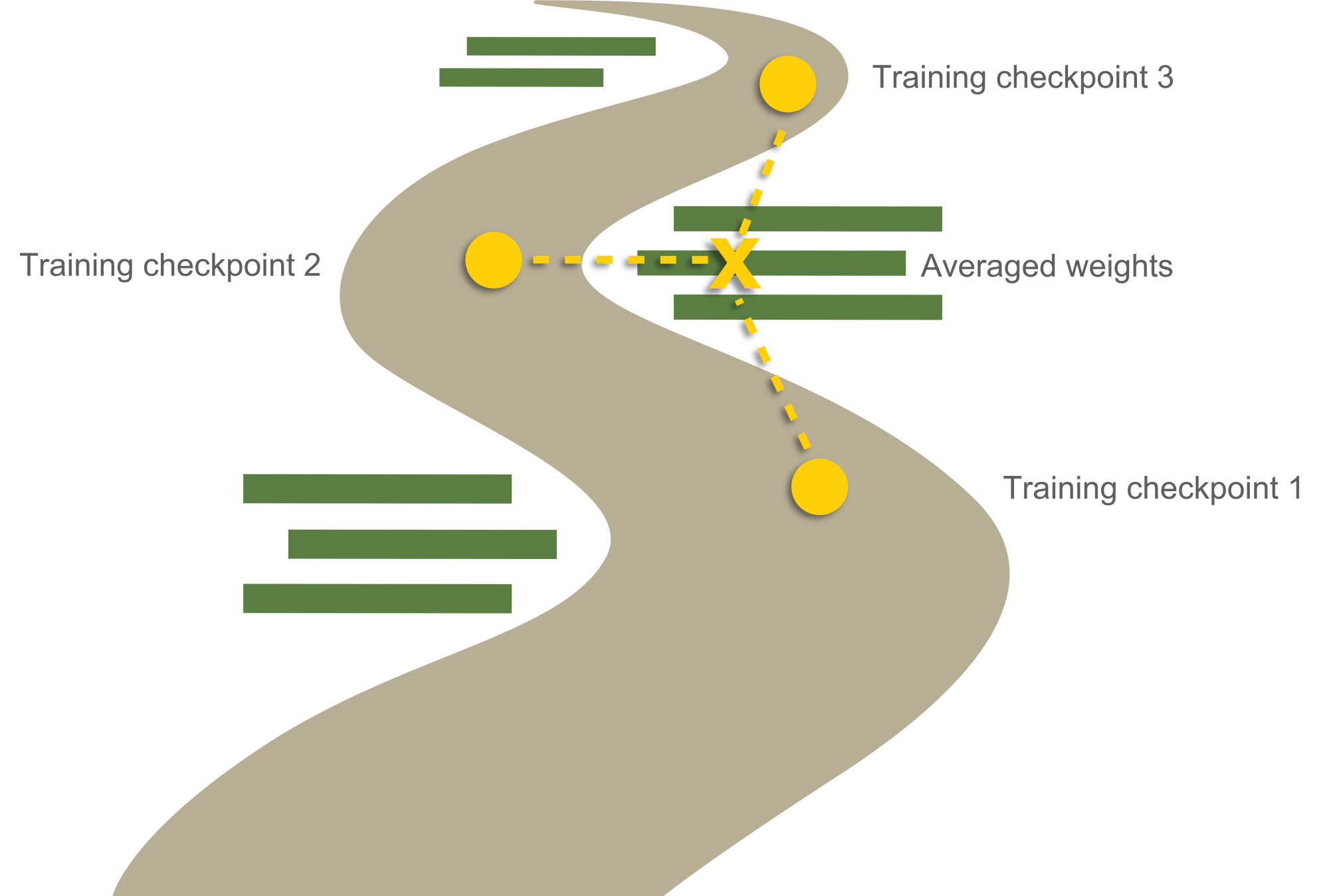
In KataGo, Wu (2020) makes use of stochastic weight averaging (SWA) (Izmailov, Podoprikhin, Garipov, Vetrov & Wilson, 2019) to generate stronger self-play training data. Experiments showed that Wu's decaying weight schedule also performed best in ChessCoach and added approximately 50 to 100 Elo in strength to networks in early training. The process of training, with thousands of weights continually being updated, is like traveling in a highly dimensional landscape and trying to find the lowest point. The SWA authors found that while the path traversed matches the training data very well, it is not the best for general and unseen data, which is what we care about during tournament play. The technique to find these better off-trail spots is almost ridiculous in its simplicity: just averaging the weights across the last few checkpoints (see Figure 13). The averaged network acts like an ensemble of networks collaborating on a decision, while still only taking one calculation.
In a call back to earlier reinforcement learning techniques, some projects have also found benefits from allowing the neural network to predict its post-search evaluation in addition to the final game result. Prasad, Abrams & Young (2018) saw gains averaging the search evaluation and the game result in Connect Four, weighting the former more heavily at the start of training and the latter more heavily at the end. Wu (2020) used a different approach in KataGo, adding auxiliary heads to the neural network with lower weight, targeting not just search evaluation but also a policy distribution for the opponent's expected reply. In ChessCoach I found that an auxiliary head and training target for MCTS value was helpful, but that a reply policy was harmful. Given the relative non-smoothness of chess, it was too painful for the network to guess badly and give a reply for the wrong move, or too difficult to shape the policy from the opponent's perspective at the other side of the board at the same time as the current player's.
Although I will leave other failures to the Development process document, curriculum learning was particularly interesting. I tried different methods of starting training with easier tasks and gradually increasing the difficulty, by blending in more free knowledge early through Stockfish evaluations and supervised datasets, and by focusing the training on the final moves of a game then extending backwards. These experiments did quite poorly. I believe this is because AlphaZero is already effectively a curriculum method. When starting out training, individual moves have negligible effect because each side is basically guaranteed to blunder any advantage, and only play accurately during the last few moves after spotting a checkmate. When training over this data in aggregate, it follows that most moves will be labelled with an equal number of wins and losses, and only clearly winning and losing moves near the end will provide consistent learning – not necessarily endgame, since checkmates may come early, but some assortment of decisive positions. The network can pick up on this new knowledge, but does not grow overconfident because of all of the noisy early-game data mixed in. In the next few games, it can see a little further ahead. It does not have to work as hard learning what it already knows, and is still encountering noisy early-game data, but there is a moving band of higher-signal data to learn. Once the network has covered different phases of the game, it is less likely to blunder advantages, and so checks, captures and tactical setups have a better chance of leading to a win. Eventually it helps to learn better openings such as the Berlin Defence; and so on. It may be that trying to tack on additional curriculum processes is not only unnecessary but hurts this serendipitous, fragile progression.
Commentary
Looking at a move or position and commenting on it is more difficult in many ways than playing chess. Generating natural language uses a specialized part of the brain that we do not intimately understand. There is no objective "best comment", and subjectively evaluating the quality of commentary engages yet more specialized brain areas on a choice of many different axes. Do we care about correctness, insight, expressiveness, personality, variety? And under which circumstances? The final comment in an article may read very differently to a standalone one. Machine learning translation commonly uses metrics such as Bilingual Evaluation Understudy (BLEU) (Papineni, Roukos, Ward & Zhu, 2002) for evaluation, and while these can be useful in context-free scenarios where there is a best answer, they can also lead to degenerate results when misapplied. On top of natural-language difficulties, high-quality commentary requires proportionate skill in, and knowledge of, chess.
An ideal way to generate lateral-language commentary would be to use a process like AlphaZero's, with a self-improving feedback cycle. However, the missing pieces may be decades away. What is needed is a comprehensive method to construct sentences and paragraphs from smaller pieces for dynamic, principled reasons; a dynamic, introspective understanding of chess concepts and writing concepts via neural network, with a search method for marrying them; and an evaluation method that considers environment context and weighs various subjective axes. This could include multiple neural networks and hand-crafted algorithms, or a single, vast network after progress in recursive thought processes, general intelligence, and meta-learning. In the meantime, researchers have started to tackle this and similar problems from various angles. Image captioning is a good place to start because it mirrors the multi-modal nature of the problem, as distinct from translation, but reaches a ceiling because dry, factual answers with little variety are intended.
Jhamtani, Gangal, Hovy, Neubig & Berg-Kirkpatrick (2018) start to break down the problem by separating chess commentary into six categories using a separate neural classifier: direct move description, move quality, comparative, planning/rationale, contextual game info, and general comment. Concentrating primarily on move quality, comparative, and planning/rationale, they train a neural network with a Long Short-Term Memory (LSTM) architecture (Hochreiter & Schmidhuber, 1997). They achieve solid results feeding in the raw position in addition to hand-crafted move, threat and score features.
Zang, Yu & Wan (2019) extend the work of Jhamtani et al. (2018), using the same dataset but training an AlphaZero-like neural network using existing game data, and specializing the commentary architecture for five of the six commentary categories. They find that using a stronger engine at the core produces better-quality commentary.
With ChessCoach I decided to take an AlphaZero-like approach by using a general architecture and feeding in all inputs in raw form, avoiding human bias as much as possible. An additional neural network, the commentary decoder, is trained using a new dataset four times as large as that used by Jhamtani et al. (2018). The network uses the transformer architecture (Vaswani et al., 2017), explained by Alammar (2018) and most recently powering the GPT-2 (Radford et al., 2019) and GPT-3 (Brown et al., 2020) systems. The transformer is powerful because of its attention mechanism, which is in some ways the opposite of the sliding mechanism of convolutional networks. Sequences can learn to focus on different parts of themselves or other sequences, regardless of distance. They can then feed this back into training a deeper understanding of the sequence elements themselves in a highly dimensional space via embeddings, explained by Collis (2017).
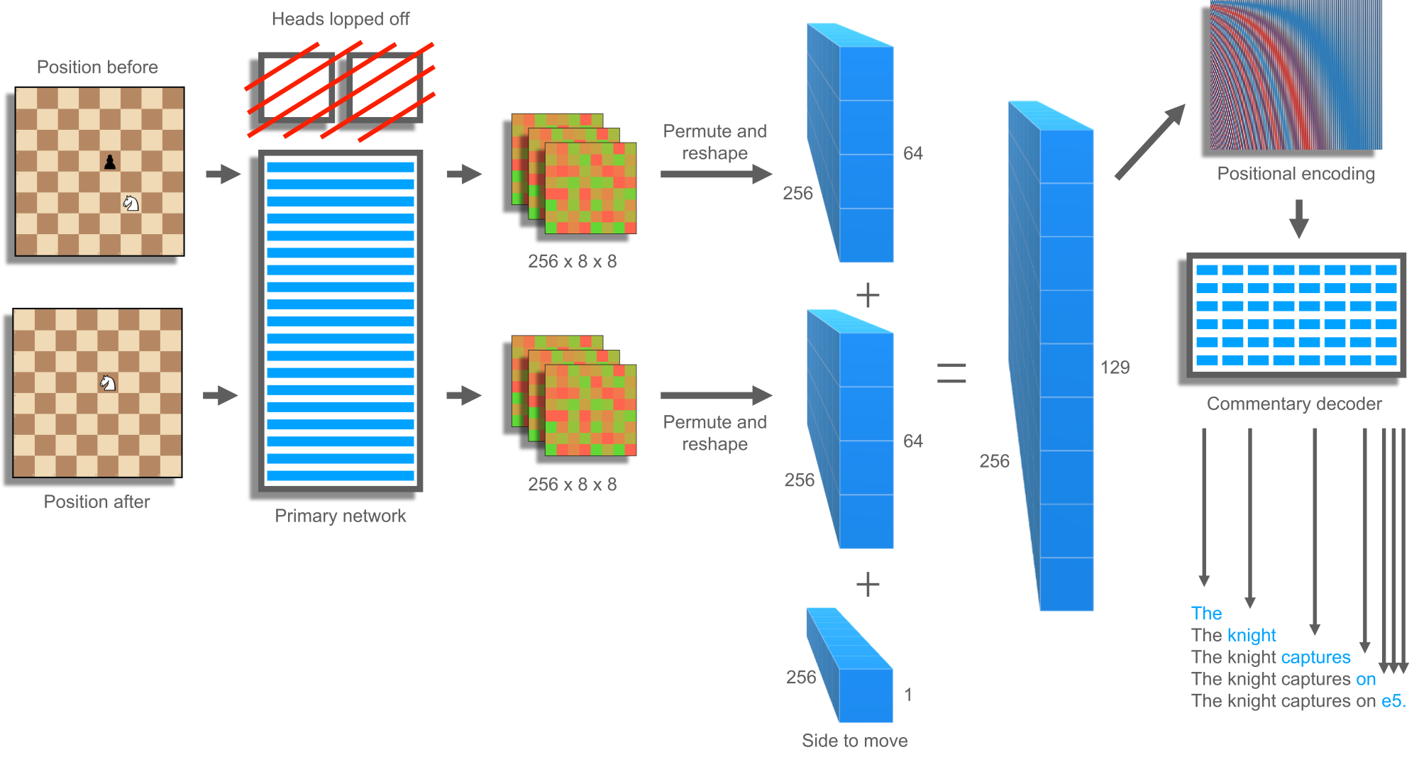
For a given chess move, the positions before and resulting from it are fed into the primary convolutional network. However, rather than taking the output of the value and policy heads, these are lopped off, and the top of the common body is taken in raw form as a collection of 256 × 8 × 8 numbers (see Figure 14). Since transformers like to deal with sequences, these are permuted and reshaped to 64 long and 256 deep, then concatenated to 128 × 256. A sequence element is appended, encoding whether it is white or black to move, since the primary model does not care, but the commentary model very much does. Then, a positional encoding like that used in the transformer paper is applied to the final 129 × 256 sequence, so that the attention mechanism of the transformer knows which position was before and which was after. Although it seems like attention alone would know about position, really it just knows about content and adds everything together. A transformer-based language model would normally tokenize the input sequence, embed, encode, decode, de-embed then detokenize. However, the current 129 × 256 sequence is arguably already embedded and encoded into a continuous space of dense chess knowledge. It is perhaps missing some details specific to the value and policy heads but contains all of the building blocks. Therefore, the input embedding and encoding portion is omitted. Experiments ratified the decision, showing that re-encoding decreased commentary quality and made the decoder unable to differentiate white and black sides.
This architecture is unprincipled in many ways, and in terms of further improvement likely offers very low-hanging fruit. The mismatch between convolutional output and sequence input feels awkward, as does the lack of self-attention in the encoder. Positional encoding is not normally applied directly before decoding. The side-to-play element is raw, not matching the rest of the encoded data. The attention mechanism with Adam training (Kingma & Ba, 2017) may be a bad fit for retraining value and policy information that was sliced off, especially without backpropagation into the primary model. Hybrid architecture, hybrid training methods or a larger commentary model, perhaps in combination with re-encoding, could help performance. Filtering out training samples that are informationless or that rely on missing environmental context could also help, at the expense of an additional trained classifier. Ideally, commentary generation would help train the primary model as a third task type. However, the two datasets are currently disjoint, with approximately 5 billion self-play positions and 1 million commentary positions: a large skew. Joint training attempts failed in ChessCoach, even considering just commentary quality, likely because the large primary model started to specialize on the narrow field of commentary positions without having enough data available to do so effectively. Using a self-play and search mechanism to generate commentary training targets would bring everything into alignment, using the building blocks listed above; however, this feels far out of reach.
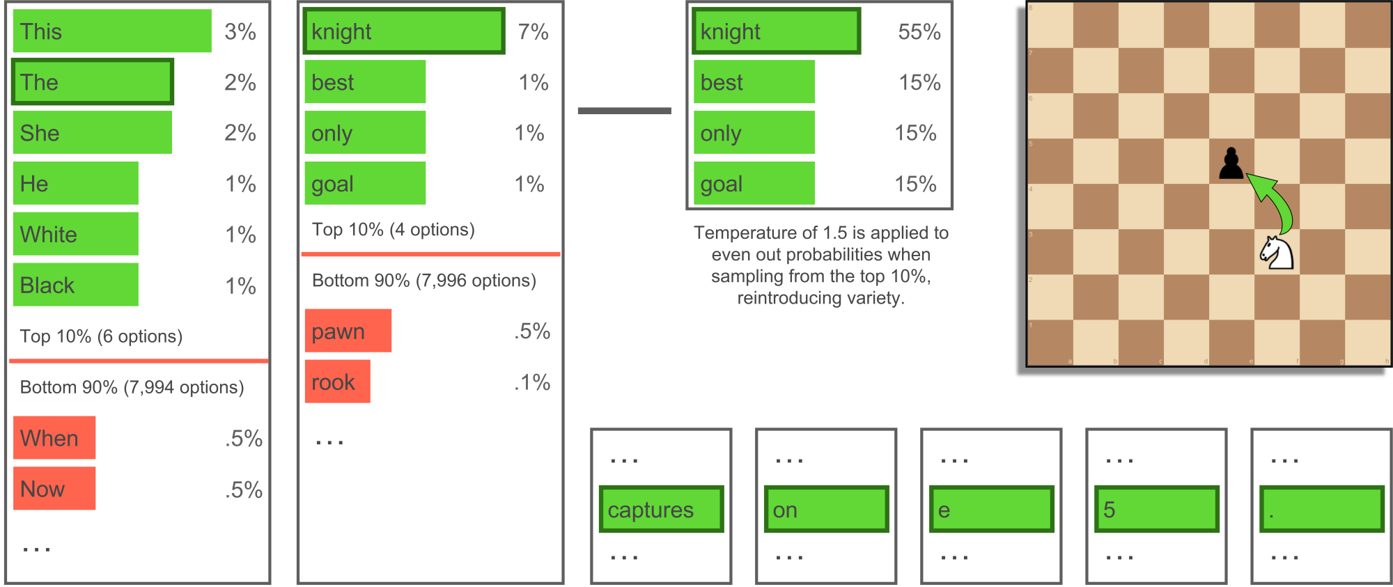
And we are not done yet! The commentary decoder does not quite give natural-language output. Instead, it outputs a set of probabilities for each vocabulary token, corresponding to a word or sub-word, after we have made a choice for earlier ones. You may sense the similarity to policy distributions, and ideally, we could again treat this as being like a PUCT search; that is, by building a tree of possible sentences or paragraphs to output and choosing the best one. However, lacking a good static or terminal evaluation function, we are forced to use alternative sampling schemes that are much less sophisticated. The most trivial is greedy sampling, which involves choosing the most likely token at each point and moving on. As you might guess from the name, this does not work too well. Next is beam search, which grows multiple writing fragments and maintains a fixed-sized set of the most likely. Looking at language statistics, it turns out that people rarely say the most likely thing, and beam search tends to give quite degenerate output outside of short translation tasks. Intended more for generative models, top-k sampling with temperature (Fan, Lewis & Dauphin, 2018) and nucleus sampling (top-p) (Holtzman, Buys, Du, Forbes & Choi, 2020) achieve much higher quality writing, especially for longer passages. These techniques have found success in state-of-the-art models such as GPT-2 and GPT-3. They achieve variety while maintaining cohesion and avoiding degeneration, and better match human language statistics, using random sampling. The top-k method randomly samples from the k most likely tokens, using a temperature parameter to sharpen or flatten the probability distribution. The top-p method randomly samples from a variable number of most likely tokens forming a probably mass p, accounting for top-k's inflexibility as distributions vary throughout sentences.
With ChessCoach I introduce a very simple variation on nucleus sampling (top-p) called COVET sampling, which focuses especially on correctness in the context of chess commentary – where the choice of rook vs. bishop and a4 vs. h7 makes a significant difference – while maintaining variety. Top-k sampling commonly uses k values of 10 to 40, and low temperature of 0.7 to 0.9, which biases towards already-more likely tokens. Top-p sampling commonly uses p values of 0.7 to 0.95 and does not apply temperature. In contrast to these norms, COVET sampling uses a low p value of 0.1 and a high temperature of 1.5 (see Figure 15). This creates a strict threshold on what can be said, but above that threshold reintroduces variety through higher temperature. Although there is occasional degeneracy – a repeated phrase or concept, or an overly long string of moves – the average and best cases are clearly improved over other top-k and top-p schemes. These particular parameters are likely closely tied to the context of chess commentary, specific dataset used, and sub-word vocabulary size of 8,000. However, the scheme of low top-p and high temperature may be equally useful in other contexts. I tried other schemes, including one I have just realized Google has tried, named sample-and-rank (Adiwardana et al., 2020), but without their SSA metric, but did not get good results. There are likely much better ideas to come that will gradually converge on generalized search as more relevant metrics are viably automated, and the field is moving rapidly.
Tournament play
Tournament play uncovers new facets in the design of ChessCoach and neural network-based engines in general. Rather than carefully optimizing for a convergent feedback cycle, the goal becomes raw playing strength. This is achieved primarily through speed, while accounting for the downsides of PUCT search and maintaining accuracy. Various techniques can be added and empirically tested using test suites and parameter optimization, given sufficient time and computing resources. As long as the techniques are turned off for self-play, have little effect within 800 simulations, or are actually beneficial for training, there is no need to worry about training targets and convergence.
Ideally, self-play and tournament play share as much code and functionality as possible, given their common search method. However, they vary most prominently in their high-level objective: self-play games per hour vs. tree nodes (positions) searched per second in one game. With self-play, it does not matter how long each game takes to finish, as long it is approximately within the space of one to two network training updates. With tournament play, as much computing power as possible needs to be directed into a single game. It is important to identify a best move in short and long time controls, and latency and freshness of information become key to the search tree growing in a healthy manner. As a result, the design of threading and parallelism between self-play and tournament play poses a challenge.
Leading classical engines such as Stockfish are well suited to modern CPUs and process millions of nodes per second. In contrast, neural network-based engines implement their models highly inefficiently compared to their biological forebears and would be limited to a few thousand nodes per second on a CPU alone. Instead, they are more suited to GPUs and TPUs, on which they can achieve hundreds of thousands of nodes per second. This is still orders of magnitude below classical engines, but with neural evaluations they are mostly competitive. It takes time to transfer data to and from GPUs and TPUs; therefore, neural network evaluations need to be processed in batches, which acts in tension with PUCT as a very sequential process, dependent on the previous result to make the next decision. Research into parallelizing tree search has provided valuable results, including virtual exploration (Liu et al., 2020) and virtual loss (Segal, 2011).
Ordinarily, a single CPU thread collecting multiple evaluations to batch, or multiple CPU threads creating larger or multiple batches, would choose the same position to evaluate many times following the deterministic SBLE-PUCT/AZ-PUCT process, undermining the purpose of batching. Virtual exploration and virtual loss allow each parallel PUCT search to choose a different position by giving a slight, suboptimal nudge to the selection process. Various dangers of doing this badly include insufficient exploitation of the best sub-trees higher up, diluting value, and over-exploitation of sub-trees lower down, again diluting value. Virtual exploration and virtual loss aim to maintain convergence towards the best move in a minimax sense by disincentivizing visits to sub-trees already being visited in parallel, with smaller relative penalties for sub-trees with many existing visits. Virtual exploration reduces the exploration incentive and virtual loss reduces the value incentive. SLBE-PUCT prevents full backpropagation when a move is especially suboptimal. Figure 16 illustrates multiple search paths being taken, with and without backpropagation. Even with these techniques to unlock parallelism, it is a challenge to efficiently coordinate multiple searches and batches and cleanly manage state while ferrying data and waiting on network evaluations.
ChessCoach uses a unified setup of N threads with M parallelism, wherein N CPU threads each alternate between performing the "CPU work" of M PUCT simulations, and performing the "GPU work" of delivering the M-sized batch of inputs and collecting the corresponding batch of value and policy evaluations. Since little CPU is used during GPU work, it can make sense to either (a) oversubscribe the number of threads relative to CPU and GPU availability, depending on the duty cycle of CPU work vs. GPU work, and/or (b) insert a multiplexing tier, with N threads doing CPU work and P<N new threads managing the GPU work. The choice of whether to multiplex depends on how efficiently the neural network library manages multiple jobs and how measurable the benefit to node freshness is as a result of faster CPU turnaround. In either case, oversubscription tends to help self-play, where node freshness is not important, but hurts tournament play, where making simulation choices based on data even a little stale because of pipelining can drastically harm tree shape and decision-making. This freshness factor makes CPU performance optimization still vital despite the system seeming GPU-bound. Other architectures are also possible with, for example, parallelism or threading creating ad-hoc batches to be evaluated. Early ChessCoach experiments showed these to have downsides in data locality or lock contention that outweighed the theoretical benefits.
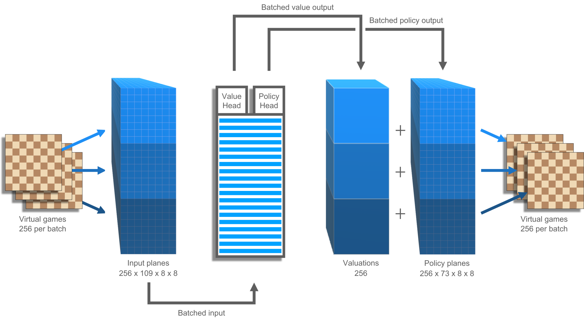
In this N-thread, M-parallelism architecture, each thread manages a fixed memory area in which network inputs and outputs are emplaced, and N × M simulations are effectively in flight simultaneously. Each thread manages M virtual chess games, each owning their own slice of the fixed memory area (see Figure 17) and operating as a coroutine, able to pause while waiting for a network evaluation and resume after. Whenever a virtual game does not need to wait, it can loop and process additional simulations. This can occur for terminal nodes such as wins, losses and some draws; for prediction cache hits, when the same evaluation has been made recently and remembered; and when using uniform evaluations before the network is minimally trained. Once all of the M virtual games are in a waiting state, the batch can be evaluated. As an example, on a v3-8 TPU, ChessCoach manages 8 threads each with 256 virtual games for a total of 2048 parallel simulations.
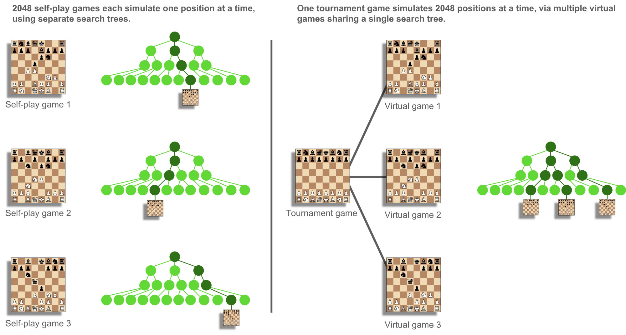
Self-play and tournament play make use of these N × M virtual games differently (see Figure 18). During self-play, each of the virtual games represents a real game with its own search tree. Since each search tree is being used entirely sequentially, no virtual exploration or loss is required despite the multi-threaded and parallel architecture, and the system is easy to manage and understand. Downsides are that individual games take a long time to finish; the initial data biases towards shorter games; and exploration is not quite as high as in AlphaZero's method without adjustments, which processed eight simulations in parallel even during self-play. In contrast, during tournament play, all virtual games are shadows of a single, real game and share a single search tree. Nodes, prediction caching and global search state all need to be processed in a thread-safe manner. Parallelism is possible without the complexity of multi-threading (1 × M) but underutilizes multiple CPUs/GPUs/TPUs. ChessCoach uses lock-free methods almost universally, relying on atomic updates and compare-and-swap instructions. Because the TensorFlow C++ API is not distributed and is not supported or documented on some platforms, to remain portable and widely readable, ChessCoach instead evaluates the neural network by calling in to TensorFlow's Python API.
With ChessCoach, I tried a variety of techniques to improve tournament strength. Again, most failed, but a few had worthwhile results. Foremost among these is SBLE-PUCT, which has additional benefits beyond those detailed in Search during tournament play when parallelism is high. With a large number of search tree nodes being evaluated per second (NPS), AZ-PUCT can grow too stubborn for two reasons. The first is that it places immense trust in its trained policy and may never explore certain tactical lines far enough to discover value, despite minutes of thinking time. The second is that even after discovering value, it may take too long for the visit count of the better move to catch up and prove its value with high certainty. SBLE-PUCT helps to overcome these flaws at high NPS by directing otherwise-wasted visits into under-explored sub-trees, and does this incrementally throughout search so that less catch-up is required. Additionally, when tuning virtual exploration and loss, and exploration incentives, there comes a point where unlocking additional parallelism starts to decrease strength because of value dilution. SBLE-PUCT can instead capture these "free" visits and explore additional sub-trees without backpropagating further up the tree.
Self-play and tournament play both use a prediction cache to remember recent neural network evaluations, but tournament play uses it more aggressively as a transposition table to save time when a position is reached in multiple different ways; for example, c4, d5, d4 vs. d4, d5, c4. Through efficient lock-free multi-threading the cache can double nodes per second (NPS) after a short time at the start position and reach even higher numbers in simpler positions. While this can give slightly incorrect value and policy when move ordering does make a difference, the speed gain compensates by allowing additional deeper evaluations.
A variety of small, specific techniques also help. These include mate-proving, faster-mate incentives, loss-prior-clearing, root-win-FPU, draw-sibling-FPU, endgame tablebase probing with bounded backpropagation, endgame minimax, exponentially weighted moving averages (EWMA), and move diversity. These are best covered in the Technical explanation.